This piece is meant to provide a brief history of Rolls science and serve as motivation toward understanding Rolls and learning how to incorporate them into any PBL study . (Since later numerical modelers, ignoring previous work, called the rolls "large eddies" in their "Large Eddy Simulations", LES, I also call rolls Organized large eddies, OLE). It should provide everything (and more) needed to understand the place of rolls in PBL modeling.
Introduction
This is a personal history of Rolls. It should be essential reading for Planetary Boundary Layer (PBL) modelers --- because if you don't know what a Roll is, your model is likely to be incorrect.
The initial impetus to the analysis that led to the mathematical description of the PBL containing Rolls came from the ubiquitous observations of cloud streets. Pictures of cloud streets were shown to me by my thesis advisor, Prof. R. Fleagle, with the comment, "Explain these for your thesis". The best of these was taken from the Apollo spacecraft showing cloud streets on the Georgia coast.
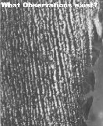 |
| An Apollo photograph from 125-mi. of cloud streets over the Georgia coast at 1500GMT on 4 April 1968. The surface flow is from bottom to top (a bottomly?), the bands are separated by about 2-km and the clouds occur at 1-km height. |
There is a fairly long history of cloud street observations, first from aircraft, then from satellites, summarized in Brown (1970, J. Atmos. Sci., 27, 742-757 and 1980, Rev. of Geophysics and space physics, 18, 683-697). An explanation for them was indicated in the 1960s by several people (e.g. Faller, Barcilon and Lilly). It turns out that the mathematically elegant Ekman solution to the Navier-Stokes equations for the PBL containing pressure-gradient, friction and Coriolis force terms, is unstable to infinitesimal perturbations. The wave with maximum growth rate has the wavelength and orientation of the cloud streets (or the streaks in Faller's rotating dishpan experiments).
But the linear instability analyses were inadequate to explain why the streets were observed to be so persistent. A linear instability analysis merely suggests that these waves grow explosively, presumably toward a breakdown of the laminar-like flow to a turbulence regime. Many assume that this simply means, back to random turbulence and a new K-theory. But there's a new wrinkle here. There's an organized flow embedded in the turbulence. Here we encounter the first of several conceptual difficulties that lead to misunderstanding of the roll solution.
The geophysical flow is already turbulent. The classical molecular-laminar solution is long gone. The turbulence has been represented by an "eddy-viscosity coefficient, K" in order to obtain mean flow solutions. In such situations we can consider that we have an "eddy-laminar" flow solution at times. Ekman's solution is an eddy-laminar solution. But now it is breaking down to another level of turbulence in the PBL. It is important to realize that the mathematics for the new regime is already burdened by the assumption that the existing turbulent eddy regime can be represented by a diffusion equation with an eddy-viscosity assumption.
In researching all `K-theory' models I came to the conclusion that this approach wasn't working very well for the PBL. There were myriad assumptions for K(z), each associated with a U(z). (Several of them started with "The problem with Ekman's solution is that it assumes a constant K, we will assume that K varies with height"; this despite the fact that Ekman also assumed a variable K, proportional to shear, in the 1905 paper.) The assumed K(z) ranged from special distributions leading to elegant Bessel function solutions to the most common procedure of simply backing out the K(z) that corresponds to the measured U(z) in the Ekman solution. (See summaries in my book --- out of print tho --- Analytic Methods in Planetary Boundary Layer Modeling, Adam Hilger LTD., London, and Halstead Press, John Wiley and Sons, New York, 150 pp, 1974. (Translated to Russian, Chinese, Korean, 1980.)
It really seemed that the observed K(z) depended critically on where and when the measurements of U(z) were being made --- there were large variations even independent of surface roughness or thermal stratification. A plot of them all looked like a can of worms, with perhaps the average somewhere near the famous "Leipzig profile" that was used for a standard for many years. Furthermore, spectral analyses revealed eddies of many sizes, with peak energies in short waves (less than 100-m), but often containing energy in selected long waves (up to PBL depth).
All this suggests that there is no steady-state Ekman-type solution. Also, it suggests that one should be wary of the eddy-viscosity concept, for it runs into conflict with the `continuum' requirement in the derivation of the Navier-Stokes equations (e.g. see Brown, Fluid Mechanics of the Atmosphere, Internat. Geophys. Series, 47, Academic Press, San Diego, 460pp, 1991).
Nevertheless, the strong correlation between the characteristics of the maximum growth rate waves of the linear solution and the observed cloud streets led me to press on for an analytic solution for the roll regime. Also, the observed U(z) seemed to be `trying' to reach an Ekman logarithmic spiral, although it never was seen exactly (except maybe occasionally in the ocean under the pack ice --- one of the few places on earth where the eddy Reynolds' number could be below critical). The cloud streets were obviously not `turbulence'. Finally, I needed a thesis topic.
The Mathematical Solution for the PBL
Why not assume that the small-scale turbulence can be represented by a K-theory and that the Ekman solution attempts to be established? Then, along the way as it establishes the turning spiral it develops inflection points in some of the velocity profiles seen in various vertical planes through the flow. A wave traveling through the PBL in a particular direction would `see' (be exposed to) au(z)/shear corresponding to the vertical profile of the U(z) in that particular direction. If a particular profile were unstable to infinitesimal perturbations, that wave would grow. Many of these profiles display an inflection point so one must check the instability of every possible profile to find the wave with the maximum growth rate. This was all done by 1968.
I assumed that the instability didn't grow into turbulence. Turbulence is characterized by randomness. The cloud streets are organized, regular, and persistent. So I hypothesized that the instability wave grew only to a certain point, where it modified the basic mean profile such that it attained equilibrium. We would then have a `finite perturbation, equilibrium secondary flow' embedded in a modified mean flow. (If I had marketing appreciation, I would have called it a `coherent' flow. A famous fluid dynamicist, H. Liepmann at Cal tech introduced this term later. I sent him my solution, upon request, in 1971. I hope it helped.)
The result of my assumptions was a "concatenation of an Ekman Solution, an instability analysis, an energy equation for the exchange of energy between the mean and the growing perturbation, and an equilibrium hypothesis (a Reynolds' hypothesis for finite perturbation equilibrium)", i.e. the perturbation was allowed to grow in the equations and the resulting modification to the Ekman solution was monitored. The energy equations calculated the flow of energy between the modified mean flow and the perturbation. Assume that when this reaches zero, we have equilibrium. Then we see what value this finite perturbation has.
As I told it, I ran the `concatenation' by walking to the computer center to load my card file, back to collect the results a few hours later, correcting the bugs twice a day. The magnitude of the instability wave (= the roll) would be u2/U ~ .002, .01, 0.9, etc. When it reached 0.07, I stopped. This was a perfect magnitude to be seen but not to destroy the `perturbation' (small) assumption for this nonlinear solution (after an Englishman, Stuart).
This might seem glib, but I had confidence. If it weren't right, there would be many observations that its predictions were wrong. So far there haven't been any. I'm still waiting, but it has been 34 years and my confidence is high. There have been many observations confirming the model's predictions.
In addition, the many assumptions that I made to reduce the stability equations to a manageable 4th order have since been relaxed. I added convection, solving the 6th order equations and Ralph Foster has added everything else, solving the 8th order equations and including thermal wind in the mean Ekman solution. The basic roll solution remains intact.
The solution yields: The modified mean flow vertical wind profile (an average over at least 10 x 10-km); the OLE, including roll winds (u,v,w)2; the convergence/divergence and mean updraft/downdraft characteristics associated with the rolls; and the lateral drift of the rolls.
The solution can be examined in a few sketches. They go a long way in explaining why one can't find a universal K(z), why profiles near each other vary significantly, why glider pilots (some of the first observers of cloud streets, responsible for their name) should be extra careful when they move from one `street' to another (there's a downdraft row in between), and why it is difficult to incorporate this solution into a numerical model.
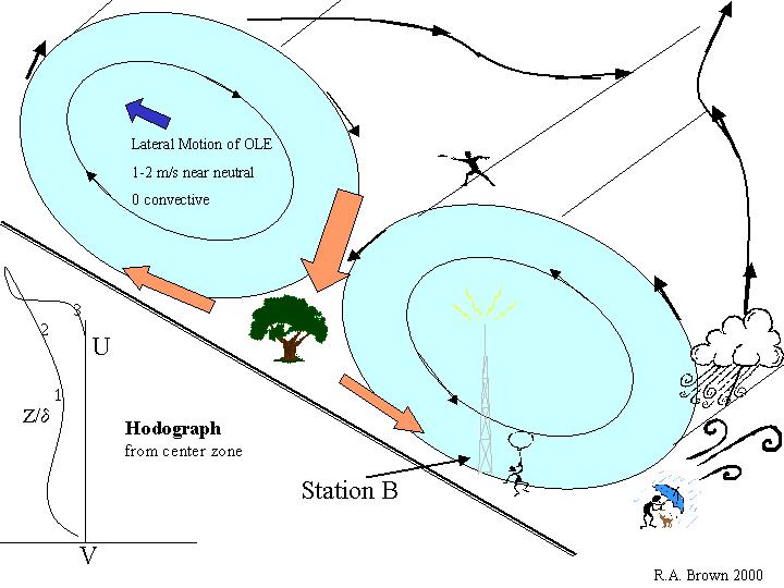
It is important to note that the solution predicts that the rolls move laterally at the mean lateral velocity at the inflection point height (about 100-m) --- about 0.07 of the PBL velocity there. This further explains the variation at a point, and why rolls in neutral stratification don't fit well in a numerical box of 5 x 5 x 2 km --- they want to drift out. Jim Deardorff (the first PBL numerical modeler) and I established this point in a conversation at NCAR in 1971. When convection becomes an important energy source, the drift goes to zero (Brown, 1972). We should have published that conversation. For some reason, later numerical modelers ignored the analytic solution (although they reproduced it in great agreement after they put the correct wavelength into their forcing boundary conditions). But they wouldn't get steady-state rolls in neutral conditions. Some reached the erroneous conclusion that the rolls existed only in convective conditions.
|
| Figure 2. |
|
| Figure 3. |
|
| Figure 4. |
|
| Figure 5. |
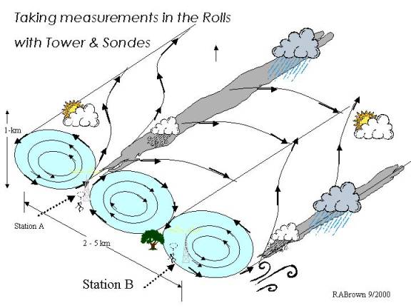
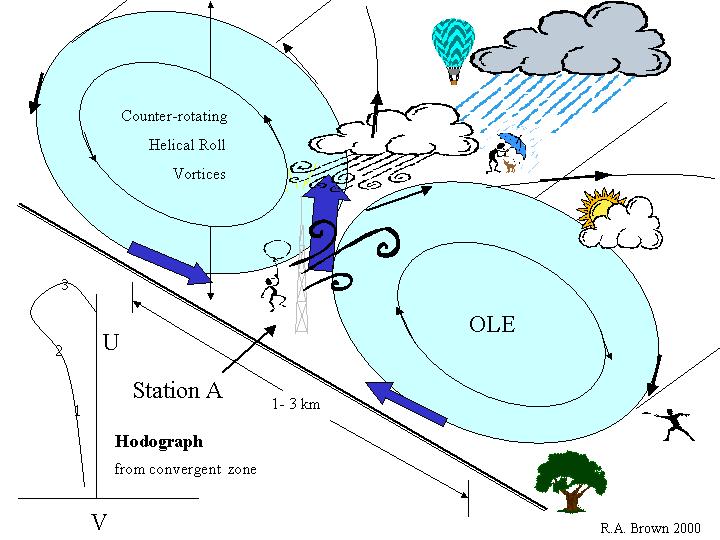
Figure 2 shows the solution for the mean flow with the organized large eddies (OLE), another name for rolls. The hodograph --- a plot of the endpoints of the vector (U,V) versus height --- shows a typical neutrally stratified layer mean profile. (6-03: at this time the hodograph is blown apart in this figure).This is the mean that would be found by averaging over many rolls (at least 10-km perpendicular to the rolls). The angle of turning between surface wind and geostrophic is about 18 �. As seen at two representative stations in figures 3 & 4, the wind profile will vary according to where in a roll it is measured. It will also vary due to surface roughness and layer stratification --- convection and thermal wind. Near neutral stratification it will vary with time at a point. It is evident why highly variable U(z) were measured at different locations and times (recall the rolls are drifting laterally at about 1 m/s, neutral).
In the 70s, observations of tetroons (constant density balloons tracked by radar), confirmed that depending on where in the roll an observation is made, the vertical profile could be quite different. It also depended on when. The balloons would enter first one roll, then another as they were tracked drifting over 40-mi downstream. Later, Doppler radar wind cross-sections over a 2-km wide, 1-km deep section perpendicular to the mean wind showed the predicted wind pattern.Still later, lidar surface observations showed the rolls. There are in a long line of observations supporting the rolls.
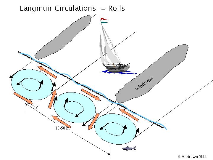
Finally in Figure 5 the solution for the ocean is shown. The PBL solution is perfectly general --- more on that later. Here, there was some controversy with wave-wave generation enthusiasts. Interaction between surface waves in proper circumstances can generate the waves in the oceanic mixed layer that produce rolls. I couldn't deny this, but showed a picture of a recently opened lead in the arctic, with pack ice in both directions suppressing surface waves. The small bits of ice were quickly gathered into rows on the ocean surface corresponding to the convergence rows of the Langmuir circulations (wind rows), suggesting they were present without the need for wave-wave interactions.
The PBL Analytic Model
My assignment in the Arctic Dynamics Joint Experiment (ADJEX), 1972-1975, was to produce a model with which to calculate the surface stress on the pack ice. My solution was to patch the nonlinear Ekman layer model to a surface layer model (Businger-Dyer) to get the U(z) from surface to geostrophic. By matching U(z) and dU/dz(z) at the top of the surface layer, a wonderfully simple drag law relation pops out, giving u*/UG as a function of a similarity parameter Hp/l, where Hp is the patch height (top of the surface layer) and d is the Ekman layer characteristic depth (= sqrt{2K/f}, where f is the Coriolis parameter).
Since neither Hp nor d can be measured very well, I didn't have much hope for this parameter. Nevertheless, plugging ahead with AIDJEX data, and assuming that this classic similarity parameter would be some function of stratification, I collected u*, zo, UG and Ta � Ts data, finding l ~ 0.15.
At this time (1973) I went to an energy transfer talk by Paul Arya where he presented the results of years' work analyzing the Australian Wangara data to determine the variation of the popular similarity parameters A and B as a function of layer stratification. They were fairly constant in unstable stratification and rapidly increased (decreased) as stratification changed to stable. These similarity parameters had been arrived at based on extrapolation of surface layer equations using dimensional analysis.
Since one of the features of the analytic patched two-layer solution was equations relating A and B to l, I went back to my office and calculated the A and B for various l. I found an excellent fit to Paul's data for a constant l = 0.17. I was surprised about the constant l, but assumed that it meant that Hp and d both increased and decreased together. This implied a quick and well mixed PBL. This might be expected when the highly efficient mixing from rolls is present.
I presented this in a subsequent energy transfer meeting. Paul could not believe (accept) that I obtained the same solution for the two similarity parameters as he had obtained with painstaking data analyses. And analytically, in an hour! Kristina Katsaros had to defend my integrity? I am certainly grateful to Paul for doing the work that established a good value for l that has lasted 25 years now. It also provided another verification that I was on the right track. The results were subsequently published but Arya chose to ignore them in his PBL book. He is not alone in ignoring the nonlinear equilibrium solution as no PBL book has presented them to this date (except mine above, and it was mainly used in Russia and Europe). Why is this?
The Consequence of OLE to PBL Modeling
The nonlinear PBL solution is complex. It provided the explanation of the cloud streets and got me my PhD in 1969. On to other things. Getting a PBL solution for relating surface stress to geostrophic winds (or surface wind gradients), for AIDJEX led to the two-layer PBL model. Naturally, since I had it at my fingertips, the nonlinear modified Ekman solution became my outer layer, the log-layer became the inner layer.
It was a scalpel for a job that required a sledgehammer. The PBL over the pack ice has such uniform stratification and surface roughness that the surface stress correlates extremely well with the geostrophic flow. This is what the model says of course, but it was lost compared to a simple correlation between geostrophic flow and pack ice motion --- they were well correlated and this does the job for AIDJEX purposes.
Higher order closure (HOC) competition
I had been exposed to higher order closure for the boundary layer in Berkeley, 1962. I was TA in a class teaching this method, which consisted of an expansion of the equations from kinetic theory, obtaining Euler's equations (zero order), Navier-Stokes equations (1st order) and the 13-moment equations (2nd order). About that time a paper was published showing that this was an invalid procedure in the boundary layer as the convergence was nonuniformly valid. Good data in the molecular boundary layer also showed that the velocity profiles from the Navier-Stokes equations were better than the higher order closure ones. We stopped teaching it.
In 1968 I again encountered HOC when John Wyngaard visited our department and presented work employing this method in PBL analysis. At a colloquium I asked how come they could use HOC in the geophysics environment when it had failed in classical fluid dynamics? He was not aware of any problem. I couldn't explain it in 2500 words or less and backed off.
Then in 1970 at an AMS Turbulence and Diffusion meeting, a panel (of Lumley, Tennekes, Wyngaard, Businger and others) was discussing HOC. From the back of the room I was considering asking my question when the guy next to me, the head of Battelle Research NorthWest, preempted me by asking the identical question. I didn't get the answer (Lumley's), but the gist was that the geophysics environment with turbulent and eddy-laminar flow was different (more complicated but easier?) than the molecular domain. HOC became very big in Atmospheric PBL modeling. The analytic nonlinear equilibrium model didn't.
Stop me if I'm wrong, but I still think that HOC is incorrect because:
- It is analytically invalid.
- It fails observationally in classical fluid dynamics (molecular boundary layers).
- It cannot represent the OLE without using wave-forcing boundary conditions and about 50 layers in a 1-km deep PBL in a 5 X 5-km box. To truly generate rolls, one needs at least a 50-km box and 50-m resolution vertically and horizontally --- tremendous computer power for a Global model.
- Relying strongly on a valid K-theory, it makes unphysical assumptions. In brief, to have a Newtonian continuum, necessary to define the mean shear dU/dz by the fundamental theorem of calculus and required in the Navier-Stokes derivation, one can have only small eddies to represent in a diffusion equation (Fluid Mechanics of the Atmosphere, R. A. Brown, International Geophysics Series, 47, Academic Press, San Diego, 460pp, Jan., 1991.)
- Observations over land have invariably revealed the roll characteristics when proper measurements and averaging were done. Observations by satellites have shown that the signature of the rolls on the surface of the ocean is ubiquitous. There is little doubt that the nonlinear solution is the correct one for the flow in the Atmospheric and Oceanic PBL. If the rolls are present, forget about K-theory and HOC for the PBL. Except perhaps as an ad hoc palliative to numerical modelers.
The Implications of the Roll Solution
The `shear' Instability
As discussed by Brown, 1980, if you have an inflection point in a flow profile you will have instabilities at very moderate flow velocities. Furthermore, if you have a situation where there is a different nearly constant flow velocity in two adjacent domains you really can't get from one to the other without encountering an inflection point in the velocity profile.� There is likewise always an inflection point in a turning wind profile. This fact can be applied to many flows at many levels in the atmosphere.Rolls can be everywhere. Even in galactic motion (with the centrifugal force a factor, as for hurricanes).
The inevitability of an inflection point occurring between two adjacent constant flow regimes was obscured a bit in the famous Kelvin-Helmholz analyses. There, the inflection point is either condensed to a point or smeared out across a layer. But it's there. In fact, in classical fluid dynamics shear is known as a stabilizing force (Jeffreys, 1928). The classic case of a constant shear layer --- Couette flow --- is notoriously stable.
As discussed by Brown, 1980, convective instability has a long history. Rayleigh did this one in 1916. Thermal instability in the presence of shear has long been known to produce rolls. If the flow is unidirectional, the rolls are parallel to this flow. This is evidently due to the fact that shear suppresses instabilities trying to grow in the shear direction. Those trying to grow laterally to the shear encounter no such suppression and appear first (have maximum growth rate). This happens a lot in geophysical flows.
The Shear-Convection Instabilities Interaction
For a long time I looked for the transition between dynamic and convective instabilities in the equations. I figured that since the dynamic instability appeared when Re > some critical number, mainly based on flow velocity, and convective instability appeared when Ri (or Ra) > critical, mainly based on vertical temperature gradients, some mixture of Re/Ri should yield a critical nondimensional parameter for when the instability changed from dynamically driven to convectively driven. I knew the end points --- at Ekman flow with no convection we have ordinary OLE, and at no flow and convection we have cellular secondary flow (cells). In fact, I noted that as flow decreased to zero at constant convective forcing, the dominant instability wave would change from the characteristic roll one (wave normal to mean shear) to the case where there is an absence of a characteristic direction for the wave. In this case, dimensional analysis reveals that there has to be symmetry in the solution, hence three standing waves at 60 deg angles --- the solution for a cell.
I never found the solution for transition from `shear' (inflection point) to convective driven rolls. The `shear' instability characteristics modified with energy input from convective energy seemed to describe most rolls. { Once in 1971 I thought that I had the smooth transition from dynamic to convective mode. It was approved (at NCAR) for publication when I ran a check that didn't make sense for the convective mode. I then found that it was actually another inflection point mode higher up in the Ekman solution that my deeper boundary layer domain had allowed. Trash. }
In the emerging chaos jargon, this is what exists in the PBL:
We are analyzing a turbulent regime. We can simulate the stress force of the small-eddies with an eddy-viscosity coefficient (and get Ekman's solution) to get a rough approximation of what's happening. But it doesn't show the action in the non-horizontally homogeneous regime (10-m to 10-km). The constant eddy-laminar Ekman solution gives the wrong average flow profile.
We have the nonlinear equilibrium solution for the wind profiles in detail, with roll shape and magnitudes included, and a good modified mean prediction. This is a solution for embedded organized structure in a turbulent flow. But it's pretty complicated. Fortunately, it has been parameterized. The solution has been run for variable parameters and mean flow correlations established. There would be a hypothetical K(z) (not really a diffusivity coefficient) corresponding to the mean profile and this could be used in models. The problem arises that it would be different for different stratification, surface roughness and magnitude of U. Nevertheless, we are considering setting up a library of K(z). These are, or will be, available on the web site. Perhaps understandably, this is not enough for the numerical PBL modeler.
The rolls are `coherent structures' --- mean flow components embedded in the turbulent flow. Possibly the only analytic solution for CS. The fact that dynamically driven rolls are identical to convectively driven-in-the-presence-of-shear rolls, suggests that they are an "attractor solution" of the equations.
Observations show that strong boundary condition perturbations (flow along a cliff or over an island) tend to force energy into the rolls at the frequency dictated by the shear or convective instability. My `cute' explanation of the mixture is that the inflectional instability provides a very discrete maximum unstable wave while convection (critically depending on the ill-defined height, which is cubed, amongst other things) is very indiscriminate, choosing many waves to be unstable and is happy to pour its energy into any wave that has an advantage.
You asked about rolls and now you know more than you ever wanted to know about instabilities. Sorry. They're inseparable.
Remote Sensing Contribution
The contributions of roll theory to and from remote sensing data has proven extremely valuable to both. In 1978, we were responsible for getting good `surface truth' wind data for calibration of the SeaSat scatterometer, SASS. Our department had a North Pacific storms response observation experiment, STREX, and we subsequently participated in the Joint Atlantic Storms Interaction, JASIN, with the specific goal of obtaining good surface wind fields.
The first test was a comparison with the measured fields. Three `models' were used, the straw man --- use GCM gradient winds, turn them 20deg and multiply by 0.7; a careful synoptician's analysis (Vince Cardone) using GCM data (there were no GCM surface winds in those days) plus everything available; and our PBL model using GCM pressure fields as input. Our model won, narrowly beating the synoptic analyses. We predicted higher winds, closer to observations. Later, it became clear why we have higher surface winds. But it was a long, slow process.
High Winds
By 1990 it was clear that the UW PBL model predicted significantly higher U10 for the same UG than did the operational product from the GCMs. Susan Dickinson was working on her thesis --- evaluating the wind fields of storms as they progressed across the North Pacific using satellite scatterometer data, satellite radiometer data (SSMI) and GCM surface analyses and UW-PBL analyses based on GCM pressure fields. She came into my office and said "Bob, your model is wrong. It disagrees with the GCMs, the buoys, and the satellites." This was a common statement from my students, and I had a stock answer, "Fine. Why don't you fix it."
Years later, we finally resolved this conundrum. We decided that the UW PBL was probably right and the others were wrong. It was not really one against three. The buoy data had been used as standard for the GCM PBL model and for the satellite data. And the buoy data was routinely too low.
In over 100,000 comparisons with satellite data, Frank Wentz never found a buoy value greater than 23 m/s. We were able to find weather station ships data routinely measuring North Pacific or Atlantic storms winds > 45 m/s. There were many indications of higher winds --- on oil towers, buoys in harbors, science ships, and anemometers on islands.By 1995, several papers had affirmed the buoy deficiency in high winds due to sheltering effects (waves are huge in high winds), displacement height effects (the buoys were effectively at lower heights) and tilting effects.
In retrospect, it is pretty evident that the buoys' winds aren't very good in high winds/seas. It's just that there is no other measurement of winds. Even today, scatterometer wind algorithms are calibrated against GCM surface winds. The saving grace is that 98% of the oceanic winds are 5-10 m/s. There is still a problem with satellite model function high winds however. (See Scatterometer Observations at High Wind Speeds, Lixin Zeng & R.A. Brown. J. Applied Meteor. 37, No. 11 p 1412-1420 November, 1998; Global High Wind Deficiency in Modeling, Chapter in Remote sensing of the Pacific Ocean by Satellites, p69-77, Southwood Press Pty Limited, Marrickville Australia, pp. 454, 1998; On Satellite Scatterometer Model functions,J. Geophys. Res., Atmospheres 105 n23, 29,195-29, 205, Dec. 2001.)
Surface Pressure fields
The basic PBL model uses the geostrophic wind (aka pressure gradient) as a boundary condition to calculate the wind profile and surface stress. It was evident that the same conceptual model could use surface stress as input and calculate the UG or SP. Gad Levy took this task for his thesis work (1981) and the result was the "Inverse Model" which was used to calculate surface pressure fields from satellite data (plus a surface pressure magnitude) (Ocean Surface Pressure Fields from Satellite Sensed Winds, (R.A. Brown and G. Levy), Mon. Wea. Rev., 114, pp 2197-2206, 1986). This has proven to be an extremely valuable contribution of scatterometer data and has been revised and perfected by Lixin Zeng and Jerome Patoux (Estimating Central Pressures of Oceanic Mid-latitude Cyclones, (R.A. Brown and Lixin Zeng) J. Applied Meteor., 33, 9, 1088-1095, 1994; A Scheme for Improving Scatterometer Surface Wind Fields, J. Geophys. Res., Patoux, J. and R.A. Brown, 106, No. 20, pg 23,985-23,994, 2002; Global Surface Pressures from Satellite Scatterometers, Patoux and Brown, in press, Jn. Applied Meteor. )
The Surface Pressure (SP) fields were used to correct the MF for high winds by assuming that the pressure measurements on the buoys were still OK in high winds and using SP plus the PBL model to calculate U10. They were routinely 10% higher than the GCM products. Since the inverse pressure fields agreed well with GCM values (in the Northern Hemisphere where there were sufficient surface measurements for the GCM), I proposed that the scatterometer could be viewed as a pressure measurement instrument, and we developed a MF that successfully related SP directly to the scatterometer backscatter measurement.
On the other hand, the remote sensing data has given proof that the nonlinear equilibrium PBL solution is the correct one. The first verification came when Mike Freilich ran a UG field simultaneous with the U10 MF parameterization analysis. He noted that they were both good robust model functions and that the UG was turned 19 deg from U10 direction. The model predicts a turning of 18 deg at neutral stratification. The data suggests that the model is correct in the mean, and that the average oceanic PBL is nearly neutrally stratified.
However, the most convincing satellite data for rolls comes from the synthetic aperture Radar (SAR) data. These show that a wind MF applied to backscatter data on 100-m resolution reveal long (100s-km) lines of higher roughness/winds, roughly parallel to the wind and separated by the usual roll wavelength of 1-3-km. We obtained a NASA grant to analyze the statistics of these observations and Levy found roll signatures over 50% of the time in the North Pacific. Since I expected the downdraft regions to be sufficient to see only occasionally, the large frequency of observations indicates that the rolls are almost always there.
At the Equator
The nonlinear equilibrium Ekman layer solution has a limitation for global applications in that it relies on a basic Ekman layer to set up the turning, which provides the characteristic height for the problem. GCM modelers need a global PBL. In 2002, Jerome Patoux patched a tropics model for the PBL by Bjorn Stevens to the UW model for the remainder of the globe. This provided a global model that includes the OLE (Global Surface Pressures from Satellite Scatterometers, Patoux and Brown, J. Applied Meteor., 42, 813-826).
There is still the problem that this is mainly an analytic model. Input is simply the geostrophic or gradient wind at some height. The model then calculates the (self-similar) wind profile to the surface, the fluxes and surface stress. If air-sea temperature differences are input, the effects of stratification on the solution can be included. Horizontal temperatures input allow baroclinic effects (thermal wind) to be included in the solution. But these calculations are time consuming. E.g. if thermal wind is included, the modified Ekman mean solution with thermal wind turning is calculated and the instability mode for this modified profile is calculated to give the shape of the roll and critical wavelength. The nonlinear growth is then allowed to achieve equilibrium in the program and a magnitude of the roll is found. The modified mean flow profile is then calculated. For a numerical model, a complete library of these calculations, perhaps with a parameterization will be needed. Except of course, we are now talking about a perturbation on a perturbation, and the corrections are small.
Conclusions
Awareness of the nonlinear equilibrium solution for the PBL is essential for PBL modelers for several reasons. The rolls explain most of the troublesome variations in the observations. They provide an explanation of the observed large momentum and heat flux transport in certain conditions --- the rolls cause strong advective convergence/divergence regions with transport that is not easily modeled with diffusion coefficients. This has significant ramifications in pollution models for instance.
The PBL model has a simple concept, but a complex execution. The results are consistent and calculable for parameterization. It might be done in the next generation.