Comments on the Synergism Between the Analytic PBL Model and Remote Sensing Data

R. A. Brown
Department of Atmospheric Sciences
University of Washington
Seattle, WA 98195
rabrown@atmos.washington.edu
206 543 8438; 0308 (FAX)

Abstract

This paper is adapted from a presentation at the session of the European Geophysical Society meeting in 2002 honoring Joost Businger. It documents the interaction of the nonlinear Planetary Boundary Layer (PBL) model and satellite remote sensing of marine surface winds from the first verification and calibration studies to the current state of verification of the nonlinear model by satellite data. It is a personal history where Joost Businger had seminal input to this research at several critical junctures.

The nonlinear solution for the flow of fluid in the boundary layer of a rotating coordinate system was completed in 1969. The implications for traditional ways of measuring and modeling the Planetary Boundary Layer were huge and continue to this day. Unfortunately, this solution replaced an elegant one by Ekman that fit nicely into an hour's lecture with a stability/finite perturbation equilibrium solution that takes a semester to present. In other words, a nice paper was replaced by a book. Consequently, there has been great reluctance to accept this solution.

The first scatterometer in space was on SeaSat in 1978. Currently there are the QuikSCAT and ERS-2 scatterometers and the WindSat radiometer in orbit. The volume and detail of data from the scatterometers during the past decade is unprecedented. The value of these data depends on a careful interpretation of the PBL dynamics. The model functions have evolved from straight empirical correlation with simple surface layer 10-meter winds to satellite models for surface pressure fields. A surface stress model function is also available.

Key Words: nonlinear PBL; OLE; rolls; PBL; PBL Modelling; satellite winds

1. Introduction--- Joost Businger's Influence

In the mid-1960s, when I was a rocket scientist for Boeing, I had my first meeting with Joost and left with a fellowship to become a geophysicist. He had valuable input as I developed my nonlinear boundary layer solution at the University of Washington.

In 1977, I had finished a book delineating the non-linear solution for the Planetary Boundary Layer (PBL) (Brown, 1974) and was at loose ends. Nothing much had come of it in the USA --- there was more interest in Europe and the USSR. Professor Businger asked me to stop by the department of atmospheric sciences to talk with a NASA scientist about the feasibility of measuring surface winds from space. When I left this meeting I embarked on a career as a remote sensing scientist.

It has been very productive and this paper is a summary of the evolution of the synergy between microwave remote sensing of marine surface winds and the satellite verification of the nonlinear PBL model. This is pretty much a done deal now, and I am thinking of visiting Joost again to see what I should do the next ten years in retirement.

2. The PBL Solution

The nonlinear solution and the subsequent PBL model are well documented. They have both been used by several generations of graduate students and post-docs. Diverse observations have supported the predictions of the model. In particular, global satellite data have established the ubiquity of the solution. They have withstood the test of time.

The solution for the flow in the PBL starts with the boundary layer equations in a rotating frame of reference. These can be obtained from the Navier-Stokes equations in the classic way of Prandtl in 1905 (see Schlicting, 1960) assuming that the flow is confined in a thin layer near the surface. Or they can be taken from Ekman (1904) in his ad hoc assumption of a balance between pressure gradient, Coriolis force and viscous force. Ekman's solution to equations (1) exponentially decreases velocity with height, implying a "thin layer solution", inverting Prandtl's process.

The basic equations of Ekman are:

where velocity is (U,V), K is an 'Austauch' coefficient from the diffusion equation, ? is density and f is the Coriolis force.

The history of applications of Ekman's solution, with its inherent dependence on the eddy-viscosity assumption, was documented in Brown (1970). Also in this paper was a summary of '60s work that showed the Ekman solution was unstable to infinitesimal perturbations at Reynolds numbers (fluid speeds) that were much less than those observed in typical geophysical conditions. The instability analyses showed maximum exponential growth at wavelengths that corresponded well with atmospheric observations of cloud streets, oceanic observations of windrows and rotating dish observations of streaks.

Brown's 1970 nonlinear solution retains the advection terms, V-ÑV, adding the finite perturbation instability to the mean Ekman solution, U = U_E + u₂ where u₂ = (u₂, v₂, w₂), is the equilibrium, finite perturbation, secondary flow. The nature of the instability solution is such that all of the perturbation correlations except one vanish when integrated over a horizontal domain greater than the roll wavelength (denoted by an overbar), leaving

Here, A is a coefficient determined by the criteria for finite perturbation equlibrium (Brown, 1970).

The solution to these equations requires a concatenation of a linear solution, an instability analysis and an energy-decreed finite perturbation equilibrium. It is described in a book (Brown, 1974).

3. PBL Models

There were two methods of modeling the PBL in the 1970s, K-theory (with eddy diffusion parameter, K) and Similarity. Both assumed that the PBL was turbulent. Both recognized that the Ekman solution was unstable, in that an infinitesimal perturbation led to exponential growth.

K-theory assumed that the turbulent regime could be modeled with an eddy diffusion coefficient. A problem arose in that observations showed a myriad of vertical velocity profiles. They were matched by a myriad of K-theory distributions.

The nonlinear method of Stuart (1958) using Reynolds' energy criterion for equilibrium led to a finite perturbation equilibrium secondary flow solution (Brown, 1970). These longitudinal vortices that filled the PBL were called Organized Large Eddies (OLE) (subsequently Coherent Structures) and were explicitly described. K-theory was used for small eddies only. When this Ekman layer solution was patched to a log-layer solution a similarity model resulted. This has evolved to be called the UW PBL Model.

The nonlinear solution quickly revealed the problem with K-theory modeling when a sketch of the Rolls was presented (figure 1). The vertical velocity profile is highly non-homogeneous and frequently unsteady at a point.

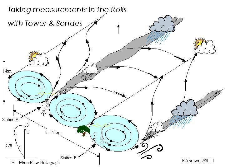
Figure 1. Sketch of the secondary (OLE) flow embedded in the mean flow (hodograph). Cloudy or clear weather correspond to updraft or downdraft regions, and the vertical hodograph could be dramatically different at stations A and B (from Brown, 2002).

Current National Weather Prediction models (NWPs) all have versions of K-theory where the eddy coefficient is chosen to correspond to the mean velocity profile. This can be the nonlinearly modified mean profile. However, this K distribution will be different for variable stratification, surface roughness and thermal wind. A complete library of carefully measured conditions will be needed to document a highly variable K.

The K-theory is sometimes produced through an approximation of a higher order closure (HOC) model. HOCs can reproduce the rolls in a numerical model (Large Eddy Simulation, LES) if the boundary conditions are carefully chosen (periodic at the sides, an integral height) and there is little lateral motion to the rolls (unstable thermal stratification). However, LES requires about 50 layers in the PBL and horizontal resolutions of 100s m. Large-eddies cannot appear in HOC models at NWP resolutions. The conclusion must be that current NWPs have the wrong PBL physics, representing advection with a diffusion coefficient, with consequent errors in PBL winds and fluxes.

For a brief period a similarity relation obtained by dimensional analysis on an extrapolated log-layer solution was used. This method determined profiles based on two or three similarity parameters. They were determined empirically (e.g. Arya, 1975). The UW two-layer analytic PBL model with a single, constant, similarity parameter reproduced these similarity parameters as functions of stratification (Brown, 1982).

My assignment for the Arctic Ice Dynamics Joint Experiment (AIDJEX) was to calculate the surface stress related to the geostrophic (or gradient) wind. This was done in Brown (1974; also see Brown & Liu, 1982). The patching of the nonlinear Ekman layer solution to the log layer solution yields a similarity law that relates u_*/U_G to h_p/d, where u_* = stress 'velocity', h_p is the patch height and d is the Ekman depth of frictional resistance, or Ö(2K/f ). The fact that neither the patch height nor d were easily measurable made prospects of this similarity relation questionable. However, observations in AIDJEX and many others suggest that a value of l = h_p/d = 0.15 was adequate across a wide spectrum of stratification variation.

The numerical modeler's reluctance to use the similarity roll model is understandable in view of the large increase in complexity of the problem. The evasion was justified in 1970 with the argument that 'Rolls are just a theory'. They were observed in dedicated airplane flights in the PBL, but these were always in cold-air outbreaks, where cloud-streets and rolls are endemic, limiting generality. For climate and weather it was assumed that an average represented by a K(z) could be used.

Some of the problems in measurements and analyses if OLE are present include:

1. The winds are non-homogeneous at the surface over a 0.1 - 5 km horizontal distance. They typically vary by ± 2 ms^-1, ± 20º in direction for a point measurement. Obtaining an average at a point can require an hour or more (see 2.).

2. Near neutral stratification the OLE move laterally with the mean lateral velocity at the inflection point height (near 100-200m). This is greatest in slightly stable stratification, decreasing at neutral stratification and rapidly near zero in unstable stratification. This explains why numerical LES models have difficulty containing the OLE in neutral stratification.

3. The PBL contains advecting flow not amenable to diffusion modeling. Numerical models cannot portray the correct physics of this mean flow without an extreme increase in resolution, vertically and horizontally.

4. The standard scatterometer and WindSat footprint diameter is 25 km. There will be about 10 OLE so the periodic effect will be averaged in satellite sensor measurements and the analytic mean flow is a reasonable prediction. This is dicey at resolutions of 6 km (scatterometer ) down to 100 m for the Synthetic Aperture Radar (SAR).

4. Scatterometry

In 1977 Joost Businger called me to a meeting in the Atmospheric Sciences Department to discuss the scatterometer soon to be launched on SeaSat. He was talking to a JPL representative, Peter Woiceshyn, about collaborating on the data analysis. Joost was the expert on the surface layer and I had just written a book on Analytic Methods in PBL modeling so Peter felt that we might add some balance to the current claims being made of winds measured from 850 km above the sea surface to an accuracy of 0.1 ms^-1.

We knew that what they were measuring with the scatterometer was the surface roughness in the 1-5 cm range (backscatter from an active radar). As any mariner knows, these capillaries and short gravity waves respond immediately to the surface wind. In fact, many sailors could discern the direction of the wind from the appearance of the waves. This is the principle of the scatterometer.

So Joost suggested that we could relate this data to u_* and thereby to U₁₀. My job as a fluid dynamicist was to determine the relation between U₁₀ and the waves. I knew that this appears to be an intractable problem with no available analytic solution. But it didn't matter if the empirical correlation was adequate.

A scatterometer doesn't measure winds. It measures capillaries and short gravity waves that are related to z_o and u_* in some unknown way.

Fortunately, there exists a relation (e.g. Fleagle & Businger, 1980):

U₁₀/ u_* = F ( z, z_o, stratification?). (3)

This was established over land and assumed to be true over the ocean. It suggests that a relation may exist between U₁₀ and u_* and z_o - hence the backscatter. What was found in 1978 as the SeaSat data came in --- for 99 days --- was an excellent correlation between the backscatter off these waves and the magnitude and direction of the surface wind. It was not accurate to ± 0.1 ms^-1, but ± 2 ms^-1 was a joy to work with. It has been verified in the 25 years since Seasat.

At first I was skeptical. I sympathized with the many excellent reasons why this correlation could not be robust. In my first paper (Brown, 1983) I started by listing ten reasons why this could not work. Then I showed the correlation data. It worked.

In that paper it was shown that we could locate atmospheric fronts to within the 50-km footprint accuracy. This has evolved to a 25-km, or less, distance. The study of fronts in exquisite detail can be found in Patoux (2003). These results have inspired some numerical modelers to increase the resolution (about 35 km) to the point where fronts appear in the numerical models. However, in numerical weather prediction models, when the best resolution is still above 35 km, a majority of fronts in the tropics and Southern Hemisphere are currently miss-placed by an average of 120-km.

5. The Pressure model function

There is an easy extrapolation of the arguments for equation (3) to:

Fortunately, there exists a relation (Brown, 1974):

U_G/ u_* = F (z, z_o, stratification, l , ??). (4)

This relation was established as the University of Washington PBL model, UW PBL_LIB (http://pbl.atmos.washington.edu) and verified in 20 years of comparisons between satellite scatterometer derived pressure fields and those of NCEP and ECMWF. The modified Ekman layer (two-layer similarity) model has been patched to a tropical PBL model (Stevens, et al. 2002) to provide a global similarity model.

The evolution of this model function was to first invert the UW PBL model to take surface wind (or stress) as a boundary condition and yield geostrophic (or gradient) wind as a product. The pressure gradients can be calculated from U_G and assumed to be impressed on the surface (Levy, 1987). The magnitude of the pressure is provided by a surface measurement or optimization techniques. The equations include corrections for stratification, surface roughness and thermal wind.

These pressures were compared to ECMWF pressure fields and found to agree within a ± 1-2 mb, an indication that the PBL model was doing well. Storms in the Northern Hemisphere were closely correlated. However there were significant differences in the tropics and southern hemisphere, with the numerical forecast model (ECMWF) missing 25% of the storms entirely. The difference probably had something to do with the extreme sparcity of ship reports compared to the constant density of satellite data there. Improvements in the numerical model resolution and the use of satellite scatterometer data for re-initialization have improved the situation such that, from a survey of 102 storms in 1996, 25% were good matches (-3 mb mean diff.), 70% had good magnitudes but were misplaced by an average of 280 km, and only 5-10% were missed entirely in the southern hemisphere and tropics. The scatterometer up there right now, QuikSCAT, misses none.

Since the surface pressure measurements are more reliable than surface winds, particularly at high winds, Zeng & Brown (1998) used buoy pressure data as 'surface truth' to establish U_G, sP and U₁₀ . These U₁₀ were compared to those from the model function (MF) for the NASA scatterometer NSCAT on the Japanese satellite ADEOS-I and a correction to higher winds was found. This was incorporated into the NSCAT MF.

The success in obtaining accurate surface pressure fields with the inverse PBL model suggested that a correlation between the sensor signal (s_o ) and sP from NCEP and ECMWF analyses products would work. Success of such a scheme depended on a large-scale comparison of s_o and sP. There would have to be a well-defined sinusoidal variation corresponding to wind directional effects on s_o . The results, shown in figure 2, indicated that the direct pressure MF (PMF) was viable. The curves are obtained in a curve fit to thousands of points of comparison between sensor backscatter and observed wind speed and direction. The peaks represent upwind and downwind backscatter values for the given bins for wind speed and incidence angle of observation. There is a small but sometimes distinguishable difference in upwind and downwind signal. The troughs represent cross-wind values. There is clearly a discernable wind direction signal that is as strong for V_G as it is for U₁₀.

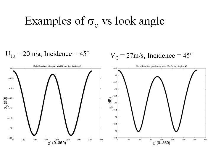
Figure 2. Quality of MF correlations for U₁₀ and U_G (from Mike Freilich).

At the following QuikSCAT meeting when I suggested that the scatterometer could be a pressure-measuring sensor, some felt that I had changed from a skeptic to a starry-eyed disciple. It was said that this couldn't possibly work, because the stratification, thermal wind, ageostrophic components, and u_* sensitivity wouldn't allow it. But the PMF pressure fields that we derived from NSCAT and QuikSCAT s_o agreed remarkably well with ECMWF products in the northern hemisphere.

6. Current Status & Conclusions

In the synergistic interaction between the PBL model and the satellite data the current state of conclusions includes:

6.1. On The PBL Solution

Based on large-scale analyses of s_o from SAR data (comparable to scatterometer data at 100-m resolution), the signature of the nonlinear PBL solution for OLE is discernable on the ocean surface 50-70% of the time (the higher number if very low winds are excluded) (Levy, 2001; Beal & Pichel, 2000). Since this is an indication of minimum occurrence of OLE, this observation establishes that the nonlinear PBL solution prevails. A representative picture is shown in figure 3.

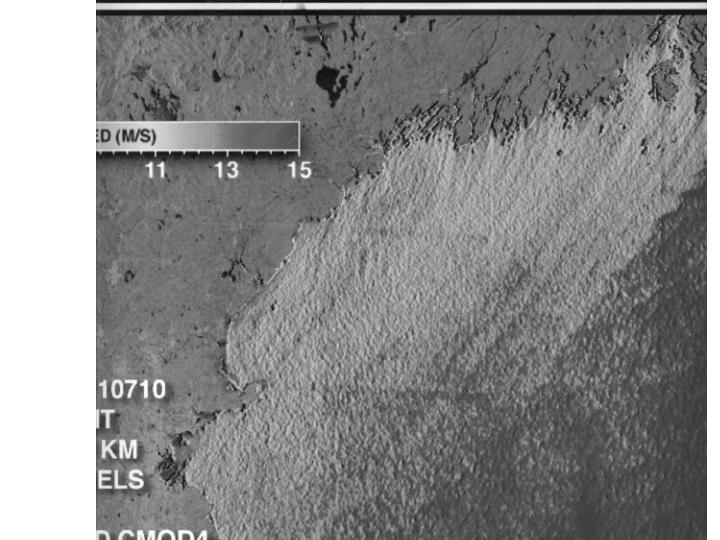
Figure 3. A portion of a figure from Beal (2000) showing winds derived from the European space Agency MF CMOD-4 for surface winds from backscatter. The wind scale shows rows of winds parallel to the mean synoptic wind (Northeasterly) with speeds of 15 ms^-1 separated from wind rows of 10-12 ms^-1 by approximately 1 km. The original figure is in color.

6.2. On The PBL Model

Observations of global ocean remote sensing data show that the nonlinear PBL solution with its characteristic OLE is a successful PBL model for relating surface winds to gradient winds and pressure fields. Current numerical analysis models all have approximate HOC PBL models (modified K-theory) where large eddies or OLE cannot be resolved. Whereas large eddies appear routinely in PBL observations, current numerical models have the wrong PBL physics with consequent errors in surface winds and heat fluxes (e.g. Foster & Brown, 1994; Brown & Foster, 1994).

A couple of remedies to this shortcoming in the numerical models can be mentioned. Either the analytic global UW PBL model (Patoux and Brown, 2003) can be substituted between U_G and the surface, with winds obtained from the analytic solution with appropriate stratification, surface roughness and thermal wind, or the analytic PBL model can be used to establish a pseudo K (z, etc.) for numerical modeling. It is possible that the LES can be used to do the second parameterization, if the problems with boundary conditions and limited domain are resolved such that the correct neutral solution can be obtained (with drifting OLE).

6.3. On Scatterometry

The satellite scatterometer provides revolutionary data to global weather and climate models. The routine daily surface winds and pressures blanket the world's oceans with data. Wind models tuned to a few buoy wind measurements are obsolete.

The SeaSat scatterometer was designed to determine surface stress. Serendipitous products for a scatterometer now include: wind vectors, fronts, surface stress vector, land vegetation, mean PBL stratification, pack ice concentration, marine surface pressure fields, storms location and strength, and mean PBL temperature.

Analysis of the scatterometer data to date have revealed that:

Storms: Are often misplaced by numerical models, are stronger (lower central pressures), and more frequent than found in numerical forecast models and climatology records.

Winds: There exist large regions of high winds (1000 km² in a storm) that do not appear in: NWP analyses buoy data, climate data or most satellite data. They do appear in the nonlinear PBL solution and some scatterometer data.

Fronts: Defined as lines of different sea state --- roughness variation --- implying a line of abrupt cyclonic change in the direction of the wind, are ubiquitous, persistent and reveal different behavior through their life cycle.

Other revelations for the PBL from scatterometry include: Correspondence between scatterometer derived and NWP analyzed 'Surface Truth' pressure fields indicate that both scatterometer winds and the PBL model are accurate within ±2 m s^-1 RMS. The 3-month, zonally averaged offset angle (U_G, U₁₀) of 19° suggests that the mean marine PBL state is near neutral. Mean swath deviation angles can be used to show thermal wind stratification (Foster et al., 1999). Higher winds (than NWP models or buoys) from pressure gradient fields agree with large eddy effect predictions. Surface pressure fields (or V_G ) rather than U₁₀ should be used to initialize NWP models. This has been done successfully in the Goddard numerical forecast model (Robert Atlas, personal communication) and the Japanese numerical forecast model (A. Nomura, personal communication).

6.4. On Surface 'Truth'

Ship winds have poor surface winds due to blockage and variable height effects. When carefully calibrated with respect to neighboring buoy or tower data, some dedicated met ships have adequate surface wind measurements.

Buoy winds are often not good surface truth. There are no measurements of U₁₀ > 23 ms^-1 in 100,000 comparisons with satellite data. Errors are due to tilting, displacement height,

sheltering and variable buoy height effects. NWP PBL models that have been tuned to buoy winds remain ad hoc models, with too-low winds and unphysical response to stratification, roughness and thermal wind.

6.5. On Satellite Surface Wind Sensors

There exist model functions for winds and pressures from satellite scatterometers (QuikSCAT, SeaWinds, ERS2) correlated to global buoy data and global NCEP surface analyses. There are winds (speed and perhaps vectors) from radiometers (WindSat) correlated to buoys; wind speeds from SARs, altimeters, and radiometers; and direct atmospheric winds from lidar measurements --- a Doppler vector wind return (so far, only on aircraft).

References

Arya, S.P.S., 1975, 'Geostrophic Drag and Heat Transfer Relations for the Atmospheric Boundary Layer', Quart. J. Roy. Meteor. Soc., 101, 147-161.
Beal, R.C., 2000, 'Toward an International Storm Watch Using Wide Swath SAR', Johns Hopkins APL Technical Digest, 21, 1, 12-20.
Beal, R.C. and W.G. Pichel, 2000, 'Coastal and Marine Applications of Wide Swath SAR', Johns Hopkins APL Technical Digest, 21, 1.
Brown, R.A., 1970, 'A secondary flow model for the planetary boundary layer', J. Atmos. Sci., 27, 742-757.
Brown, R.A., 1974, 'Analytic Methods in Planetary Boundary Layer Modeling', Adam Hilger LTD., London, and Halstead Press, John Wiley and Sons, New York. 150 pp.
Brown, R.A., 1982, 'On Two-Layer Models and the Similarity Functions for the Planetary Boundary Layer', Bound. Layer Meteor., 24, 451-463.
Brown, R.A., 1983, 'The Scatterometer as an Anemometer', J. Geophys. Res., 88, C3, 1663-1673.
Brown, R.A., and T. Liu, 1982, 'An Operational Large-scale Marine Planetary Boundary Layer Model', J. Applied Meteor. 21, 3, 261-269.
Brown, R.A., & G. Levy, 1986, 'Ocean Surface Pressure Fields from Satellite Sensed Winds', Mon. Wea. Rev., 114, pp 2197-2206.
Brown, R.A., Ralph Foster, 1994, 'On PBL Models for general circulation models', The Global Atmos.-Ocean System, 2, 163-183.
Brown, R.A., 2000, 'On Using Satellite Scatterometer, SAR and other Sensor Data and Serendipity', Johns Hopkins APL Technical Digest, Vol. 21, #1, 21-26.
Brown, R.A., 2001, 'On Satellite Scatterometer Model functions', J. Geophys. Res., Atmospheres, 105,, n23, 29,195-29,205.
Brown, R.A., 2002, 'Scaling Effects in Remote Sensing Applications and the Case of Organized Large Eddies', Canadian Jn. Remote Sensing, 28, 340-345.
Drobinski, P. & R.A. Brown, P.H. Flamant, J. Pelon, 1998, 'Evidence of Organized Large Eddies by Ground-Based Doppler Lidar, Sonic Anemometer and Sodar', Bound.-Layer Meteor., 88, 343-361.
Ekman, V.W., 1905, 'On the influence of the earth's rotation on ocean currents', Arkiv. Math. Astro. Fysik., 2, 11, 1-53.
Fleagle, R.G. and J.A. Businger, 1982, 'An Introduction to Atmospheric Physics', 2nd Edition, Intl. Geophysics Series, vol. 25, 432 pp.
Foster, Ralph & R. A. Brown, 1994, 'On Large-scale PBL Modelling: Surface Wind and Latent Heat Flux Comparisons', The Global Atmos.-Ocean System, 2, 199-219.
Foster, Ralph, R. A. Brown and Amy Enloe, 1999; 'Baroclinic modification of mid-latitude marine surface wind vectors observed by the NASA scatterometer', J. Geophys. Res., Oceans, 104. n 24, 31225-31235.
Kraus, E.B. & J.A. Businger, 1994, 'Atmosphere-Ocean Interaction', 2nd Ed.,Claredon Press, Oxford, 362pp.
Levy G., 2001, 'Boundary Layer Roll Statistics from SAR'. Geophysical Research Letters. 28(10): 1993-1995.
Levy, G., and R.A. Brown, 1998, 'Detecting Planetary Boundary Layer Rolls from SAR'. Remote Sensing of the Pacific Ocean by Satellites. 128-134.
Levy, G., 1987, 'A Study of the Dynamics of Maritime Fronts Using Remotely Sensed Wind and Stress Measurements', PhD Thesis, University of Washington, Dept. Atmospheric Sciences.
Patoux, Jerome, 2003, 'Frontal wave development over the Southern Ocean', Ph.D. Thesis, University of Washington, Dept. Atmospheric Sciences
Patoux, Jerome and R. A. Brown, 2003, 'Global Pressures from Scatterometer Winds', Jn. Applied Meteor. 42, 813-826
Stevens, B., J. Duan, J.C. McWilliams, M. Munnich and J.D. Neelin, 2002, 'Entrainment, Rayleigh friction and boundary layer winds over the tropical Pacific', J. Climate, 15, 30-44.
Schlicting, H, 1960, 'Boundary Layer Theory', McGraw-Hill, 645pp.
Stuart, J.T., 1958, 'On the non-linear mechanics of hydrodynamic stability', J. Fluid Mech., 4, 1-21.
Zeng, Lixin & R.A. Brown, 1998, 'Scatterometer Observations at High Wind Speeds', J. Applied Meteor. 37, No. 11 p 1412-1420.